

Full Report
Introduction
This report, required by state law under HB3543, provides a comprehensive assessment of the state of science of climate change as it pertains to Oregon, covering the physical, biological, and social dimensions. The first chapter summarizes the current state of knowledge of physical changes in climate and hydrology, focusing on the period since the previous Oregon Climate Assessment Report (OCAR3, Dalton et al. 2017); and the second chapter covers the impacts. The second chapter is, verbatim, the Northwest chapter of the Fourth National Climate Assessment (NCA4) which was released by the federal government November 23, 2018. It is available for download separately.
The Oregon Climate Change Research Institute (OCCRI), created by the state legislature (HB3543, 2007), includes a small staff housed at Oregon State University and a larger network of over 150 researchers in Oregon and beyond. OCCRI’s vision is to achieve a climate-prepared Northwest by building a climate knowledge network, cultivating climate-informed communities, and advancing the understanding of regional climate, impacts, and adaptation.
Climate Change and Oregon
Globally, concentrations of greenhouse gases continue to rise. Last year, carbon dioxide concentrations measured at the long-term monitoring site on Mauna Loa in Hawaii exceeded 410 parts per million by volume (ppmv) for much of 2018, having topped 400 ppmv for the first time only in 2014 . Current carbon dioxide concentrations are 46% higher than they were prior to the Industrial Revolution.
Regionally Averaged Trends
Oregon’s warming trend continues. As shown in the observations in Figure 1a, after the record-warm 2015 (the recent peak of the observed temperature graph), calendar years 2016 and 2017 were also warmer than the 1970-1999 average though not as warm as 2015. The temperature of calendar year 2018 is not officially available as of this writing because the continuing lapse in federal appropriations has shuttered the official climate data analysis capabilities of NOAA. However, other sources of data indicate that 2018, too, was warmer than average.
Future warming rates will increasingly depend on global greenhouse gas emissions, as can be seen by comparing the red (high emission RCP8.5) and yellow (low emission RCP4.5) thick curves and shaded regions. The Paris agreement seeks to achieve warming no greater than 2°C, which would require that emissions track below RCP4.5; consequently, even the yellow curve and shaded region are higher than the scenarios consistent with the Paris Agreement. Annual precipitation, unlike temperature, has no long-term trend toward wetter or drier. Most recent years have been fairly close to average, with the exception of 2018, which was much drier than average based on NOAA data available in December.

Figure 1. Observed, simulated, and projected changes in Oregon’s mean annual (a) temperature and (b) precipitation from the baseline (1970–1999) under a low (RCP 4.5) and a high (RCP 8.5) future emissions scenario. Thin black lines are observed values (1900-2017) from the National Centers for Environmental Information. The thicker solid lines depict the mean values of simulations from 35 climate models for the 1900-2005 period based on observed climate forcings (black line) and the 2006-2099 period for the two future scenarios (orange and red lines in the top panel, blue and grey in the bottom panel). The shading depicts the range in annual temperatures from all models. The mean and range have been smoothed to emphasize longterm (greater than year-to-year) variability.
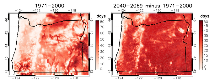
Figure 2. Projected changes in the average number of hot days (where daily high temperature >86°F, 30°C) per year. Shown are the average number of hot days per year for 1971-2000 (left panel) and projected changes by 2040-2069 assuming the high-emissions scenario RCP8.5 (right panel). Results were averaged over 20 climate models (right). Figure prepared using data on the NW Climate Toolbox, climatetoolbox.org, data source: MACA.
Spatial Patterns
Previously, we checked how well global climate models (GCMs) performed at simulating Northwest climate (Rupp et al. 2013). We then statistically downscaled 20 of the best models using the Multivariate Adaptive Constructed Analogs (MACA, Abatzoglou and Brown 2012) method. OCCRI research partner Prof. John Abatzoglou has led the construction of a “climate toolbox” in which various climate quantities are computed at fine spatial resolution for both a baseline, past dataset and for changes derived each of 20 GCMs, as well as the changes averaged over all 20 GCMs (Figures 2-3).
Figure 2 shows how ‘hot days’, defined as the days with daily high temperatures >86°F, are expected to change by mid-century (2040-2069) for the high emissions scenario. In the baseline period (1970-1999), the hottest parts of the state — lower elevation portions of eastern Oregon, as well as the Rogue River valley — experience at least 30 hot days per year. In the future, most locations except the mountains and the coast will experience at least an additional 30 hot days per year, in many places doubling the frequency of such days.
The Willamette and Umpqua valleys, along with small coastal valleys, have the longest growing season in the baseline climate, over 280 days (Fig. 3a), and the high elevations of central and Eastern Oregon have the lowest, only a couple of months. By mid-century in the high-emissions scenario (Fig. 3b), most of western Oregon would see a lengthening of the growing season by about two months. Some of the higher elevation locations in central Oregon would also see a lengthening of about two months, and the rest of the state would see lengthening of about a month. Accompanying these changes is a shift by over a month later in the date of first fall freeze in the highlands of central Oregon (Fig. 3d) and a shift by over a month toward earlier date of last spring freeze in much of western Oregon (Fig. 3f).
To augment the information from GCMs, OCCRI also runs a fine-scaled (25 km) regional model to more accurately simulate the physical processes associated with topography like mountains which influence the responses of the atmosphere (and hence temperature and precipitation) to rising greenhouse gases. Our approach uses a crowd-sourced climate modeling platform to generate a ‘superensemble’, that is, a very large collection of simulations that allows better statistical representation especially of extremes (Mote et al 2015).
Figure 4 shows the seasonal mean changes in temperature from this regional modeling superensemble. These results are for the lower-emissions RCP4.5 scenario, which by mid-century (2030-59) is noticeably lower than RCP8.5. In winter and spring, warming is 10-20% larger in the mountains, especially the Sierras and the Cascades, than in surrounding areas. Analysis indicates that ‘snow-albedo feedback’, in which modest warming is accentuated where snow disappears, is primarily responsible for these changes. In the Northwest (see Table 2.2 of Dalton et al, 2017) as well as globally, the ocean warms less than land. As with many GCMs, our regional model projects larger warming in summer, which leads to sharp spatial contrasts between land and ocean warming across the coastal mountains. In other words, Oregon’s coastal areas will only warm about 0.4°F (0.2°C) per decade, the rest of western Oregon around 0.7°F (0.4°C) per decade, and eastern Oregon more than 0.9°F (0.5°C) per decade. Similar patterns are visible in fall, though with smaller magnitudes.
For precipitation (not shown), both the set of global models and our regional model suggested modest increases in winter precipitation and modest decreases in summer precipitation. In addition, our regional modeling results for mid-century suggest a weakened rain shadow effect in winter, with larger increases (>20%) in precipitation east of the Cascades and small (<10%) increases west of the Cascades. These changes in seasonal means are matched by changes in extreme precipitation (Figure 5) which are relatively larger east of the Cascades. For example, the 99th percentile (wettest day in 100 days) goes up 6% west of the Cascades but 14% east of the Cascades.
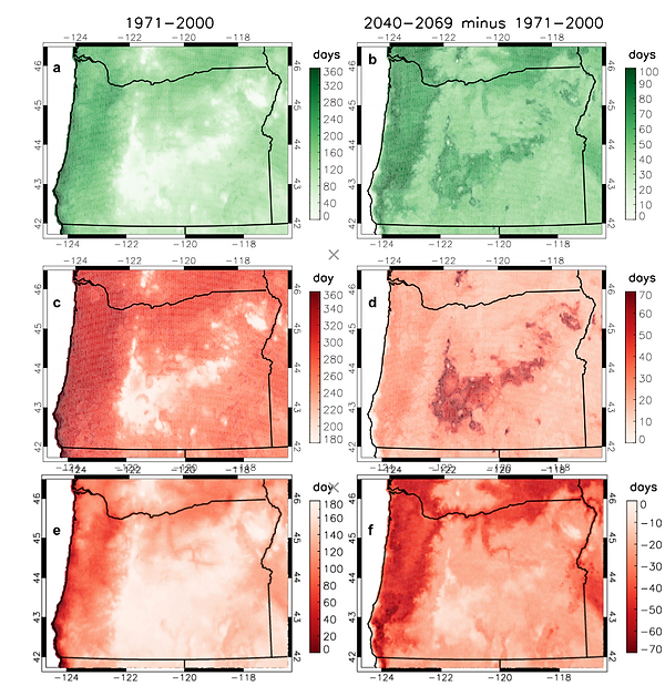
Figure 3. Baseline (left column) and projected change from baseline to mid-21st century for RCP8.5 (right column) in growing season (top), defined as the number of days with daily minimum temperature (Tmin) > 32°F (0°C); date of first fall freeze (Tmin<32°F, middle); and date of last spring freeze (Tmin<32°F, bottom). Results were averaged over 20 climate models; from data on the NW Climate Toolbox, climatetoolbox.org. Data source: MACA.

Figure 4. Projected change in mean temperature, 1985-2014 to 2030-59, from a regional superensemble using the low (RCP4.5) emissions scenario for (a) Dec-Jan-Feb (winter), (b) Mar-Apr-May (spring), (c) Jun-Jul-Aug (summer), and (d) Sep-Oct-Nov (fall). Adapted from (Rupp et al. 2017) and used by permission.
Hydroclimate
Since OCAR3 (Dalton et al. 2017), a new analysis of observed changes in snow resources in the west (Mote et al. 2018) show that nearly every location in Oregon experienced declines in spring snowpack since mid-20th century. Recently, an analysis of atmospheric variability (Siler et al 2018) indicates that the influence of regional warming on the west’s snowpack since 1985 has been largely masked by natural variability in ocean temperatures and atmospheric circulation patterns important during the cool season, effectively slowing the rate of spring snowpack decline. The authors expect greatly enhanced response in the snowpack to warming in coming decades as this pattern ebbs.
The climate toolbox depicts how the region’s water variables will change. For example, Figure 6 shows the disappearing snowpack expected by the end of the century. Most of the Northwest will see decreases in April 1 snowpack in excess of 56% but the highest peaks in the Cascades are projected to decrease less, only in the 11-33% range. These reductions in snowpack will lead to wintertime increases but summertime decreases in soil moisture in most places (Figure 6). The increases in soil moisture in the driest parts of the region are also seen in the regional superensemble, and are confined to lower soil layers. Upper soil layers also dry substantially there, but the paucity of deep-rooted plants limit the depletion of lower soil layers.
In most basins, the changes in snowmelt timing also alter streamflow (Figure 7). The increases in average wintertime flow (owing to reduced snow accumulation and more rapid runoff) also correspond to increases in flood risk in those basins. Summertime flow is reduced in many basins, by as much as 50% (in June).

Figure 5. Simulated extreme one-day precipitation are shown by percentile for western Oregon and Washington (left) and eastern Oregon and Washington (right), for 1985-2014 (black) and 2030-59 (red). For example, the 99.9th percentile is the wettest day in 1000 days. Figure from Li (2017) using weather@home data.
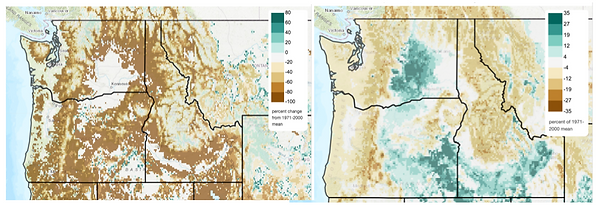
Figure 6. Change in (left) April 1 snow water equivalent and (right) summer soil moisture, for 2040-69 under the high-emissions RCP8.5 scenario, as a percentage of 1971-2000 baseline from a mean of 10 GCMs. Figure prepared using the NW Climate Toolbox, climatetoolbox.org.
Data source: VIC hydrologic model.
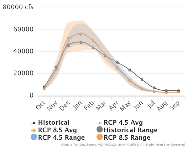
Figure 7. Monthly non-regulated streamflow in the Willamette River at Salem for 2040-2069 under high and low emission scenarios and over the 1971-2000 historical baseline. Shaded regions show the range from 10 climate models. Figure prepared with the NW Climate Toolbox, climatetoolbox.org, data source: streamflow routing of VIC hydrologic model.
Fire-climate risk
Placing weather-related events in a historical context can be a useful exercise, especially when trying to understand the meteorological conditions that certain hazards, e.g. wildfires and drought, favor and how these events may be exacerbated by changing climate. Wildfires have received considerable attention over the past two years, due to their devastation (Camp and Carr Fires in California; Substation Fire near The Dalles) or economically or socially valued location (Eagle Creek Fire in the Columbia River Gorge and Chetco Bar Fire in southwestern Oregon). Statistical analysis shows that warm, dry summers are associated with higher area burned (McKenzie et al 2004, Westerling et al., 2006). Large fires increased in the western US from 1984-2011 in a warming climate (Dennison et al., 2014) and human-caused climate change was responsible for the increase in area burned in forests in the western US from 1984-2015 (Abatzoglou and Williams, 2016).
Fire season in Oregon runs roughly from late July to mid-September, though it can start earlier and end later, as was the case in 2018. Fire activity is dependent on many anthropogenic and natural variables, and warmer or drier seasons can create conditions favorable for wildfires. In Figure 8 we define fire season using a rough definition of the months of July-September. The upper left quadrant represents the warmest and driest years in this historical record; the lower right quadrant shows the wettest and coolest years. Years for the climate analysis are only labeled from 2002-2018, the same period of record as the fire data, to reduce clutter. Circles are meant to show the acres burned in each of these years, binned into groups.
The fire seasons with the most acres burned (2012, 2014, and 2017) are among the warmest in the record, and notably warmer than most of the other years in the upper left quadrant. July-September 2012 and 2017 were drier than normal, but the same time period in 2014 was slightly wetter than the historical average. There are years (2003, 2009) that were in the top 10 warmest July-Septembers on record, but had relatively small areas of wildfire activity. 2002 and 2012 had significant large fires (over 500,000 acres) boosting the overall total; the 2002 Biscuit Fire in southwestern Oregon and the 2012 Long Draw fire in eastern Oregon. Both fire seasons topped 1,000,000 wildland acres burned. 2010 had near-normal precipitation and temperature and 2004 was wetter than normal for the fire season; these two years had the smallest area burned on record. In this typically arid season in Oregon, a few rainfall events can skew the entire season. 2013 was notable as it was Oregon’s wettest September on record, owing to two large storms early and late in the month. July-September has consistently been warmer and drier than the 1895-2018 average for most of the past 17 years, creating prime conditions for potentially large wildfire seasons. And while large wildfire seasons can be dominated by single events, warmer conditions tend to be more favorable for an above average area burned in Oregon, consistent with the rest of the western US. None of the years with above-average area burned were near normal in seasonal temperature and precipitation. In a changing climate, fire activity in Oregon will continue to be influenced by warming temperatures and longer fire seasons. Projections using vegetation models (previously published in OCAR3, Dalton et al. 2017) highlighted spatial differences in changing fire risk, emphasizing that more frequent fires could be expected even in the wet western third of the state, and indeed as the Eagle Creek fire (summer 2017) showed, that prediction is coming true.
Weather data can be used to calculate fire risk in various ways. Operational agencies often use the energy release component (ERC) as well as measures of fuel moisture and wind speeds. One measure of the fuel moisture is the ‘100-hr’ fuels moisture, which is the amount moisture within vegetation (the ‘fuel’), averaged over 100 hours. Figure 9 shows the ‘100-hour’ fuel moisture, specifically the number of days per summer when the fuel moisture is below the 3rd percentile (“extreme”). The largest increases in the frequency of extreme fire risk are in the eastern third of Oregon and in the Willamette Valley.

Figure 8. Scatterplot of fire season (July-September) mean precipitation and temperature, with area burned in each year since 2002 indicated by circles. Climate data are from NOAA’s National Center for Environmental Information statewide data for Oregon for 1895-2018 (the average for this entire period is used to calculate anomalies). Wildland fire data for 2002-2017 are from the National Interagency Fire Center (NIFC). Preliminary 2018 data are included here, but the final figure was not available from NIFC due to the lapse in federal appropriations. Prescribed fires were excluded from the analysis.

Figure 9. Projected change in extreme fire risk days, defined as the number of days when the 100-hour fuel moisture in June-July-August (JJA) is below the 3rd percentile of days in the baseline period. Figure prepared with data on the NW Climate Toolbox, climatetoolbox.org. Data source: MACA
Sea level rise: long term view
Projections for sea level rise to 2050 have not changed substantially in recent years, but new estimates of the maximum physically plausible sea level rise by 2100 are now 8.2 feet (2.5m) (USGCRP 2017, p. 343). Intermediate estimates are also higher than some previous assessments, 3.3 feet (1.0m) by 2100. Moreover, an improving understanding of the behavior of the Antarctic ice sheet especially in past glacial-interglacial cycles has advanced the understanding of its future response to warming. A crucial point about both Greenland and Antarctica is that even after global temperatures are stabilized, melting will continue until a new equilibrium is reached. In the case of Greenland, there is growing concern that any warming beyond 1.5-2°C could lead to the irreversible melting of the entire ice sheet: once the melting reduces the altitude enough, the ice sheet cannot accumulate enough new snow in winter to offset the melting in summer. In the case of Antarctica, recent research by Oregon scientists (Clark et al. 2018) shows that the equilibration to a new climate would take thousands of years. Their analysis suggests that stabilizing global climate at 2°C above preindustrial would limit sea level rise to less than 3.3 ft (1m) by 2300, but even so, it could reach 9m by the year 9000. Higher emissions scenarios could lead to increases in global mean sea level of almost 10m by the year 2500 and over 50m by the year 9000. The authors note that the policy consequences of limiting emissions now will last for millennia.
Potential surprises
The Climate Science Special Report includes a chapter (Kopp et al. 2017) on potential surprises, compound extremes and tipping elements. The key findings are worth paraphrasing here:
-
Positive feedbacks (self-reinforcing cycles) within the climate system have the potential to accelerate human-induced climate change and even shift the Earth’s climate system, in part or in whole, into new states that are very different from those experienced in the recent past (for example, ones with greatly diminished ice sheets or different large-scale patterns of atmosphere or ocean circulation). Some feedbacks and potential state shifts can be modeled and quantified; others can be modeled or identified but not quantified; and some are probably still unknown. (Very high confidence in the potential for state shifts and in the incompleteness of knowledge about feedbacks and potential state shifts).
-
The physical and socioeconomic impacts of compound extreme events (such as simultaneous heat and drought, wildfires associated with hot and dry conditions, or flooding associated with high precipitation on top of snow or waterlogged ground) can be greater than the sum of the parts (very high confidence). Few analyses consider the spatial or temporal correlation between extreme events.
-
While climate models incorporate important climate processes that can be well quantified, they do not include all of the processes that can contribute to feedbacks, compound extreme events, and abrupt and/or irreversible changes. For this reason, future changes outside the range projected by climate models cannot be ruled out (very high confidence). Moreover, the systematic tendency of climate models to underestimate temperature change during warm paleoclimates suggests that climate models are more likely to underestimate than to overestimate the amount of long-term future change (medium confidence).
All of these points are highly relevant for Oregon as it considers policies to reduce emissions and prepare for future challenges to its climate-sensitive natural resource economy, natural world and cultural heritage, infrastructure, health, and frontline communities. These are covered in the Northwest chapter of NCA4, available here.